What is procedural programming?
INFO
Python allows for object oriented, procedural, and functional programming models, or as they’re often called paradigms.
The main purpose of a programming model is to structure your code.That structure makes it easier to update the code and create new functionality within the code. But there’s no one perfect model that’s a solution to coding structures, and sometimes a combination of approaches works best.
Procedural programming structures code into procedures, sometimes called subroutines or functional sections of code.
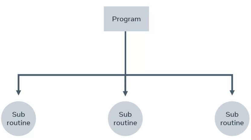
Because of this approach, the code is made up of logical steps to complete a specific task.
For example, adding two numbers to return their sum. I can add together the numbers 5 and 10 with a short piece of code. Now I want to add together the numbers 8 and 4. However, the code I wrote was specifically to add 5 and 10. For my new numbers, I must create another similar piece of code to do the calculation. That would not be a very efficient way to code.
Instead, I changed the code into a function that will accept two numbers as arguments and return the sum.
I now have the function called sum, which can be re-used as many times as I like with many different sets of numbers.
DRY
In programming, there is a principle called DRY. Don’t repeat yourself. It’s all about reducing duplication in code.
A guideline to keep in mind is to create functions that can be reused throughout your application.
In summary, the advantages of the procedural paradigm are:
- It’s easy for beginners to learn and get started.
- Procedures can be reused by other parts of the code.
- Code is easy to understand because each procedure is broken into specific tasks.
Disadvantages:
- It can be hard to maintain and extend.
- In some cases, it doesn’t relate well to real-world objects.
- Data is exposed throughout the whole program.
Algorithms
Algorithm
An algorithm is a series of steps to complete a given task or solve a problem.
In programming, algorithms are used to solve a multitude of problems that range from simple to very complex. The key to understanding and creating an algorithm is to break the problem into smaller parts.
Examples
I’m going to demonstrate a particular algorithm that checks if a word is a palindrome. A palindrome is a word that can be spelled the same, both backwards and forwards.
# My code
print("This program checks if a word is palindrome.")
x = input("Please enter a word: ")

isPalindrome = True

for i in range(int(len(x) / 2)):
    if x[i] != x[len(x) - i - 1]:
        isPalindrome = False
        break

if isPalindrome:
    print("Yes")

else:
    print("No")
# Algorithm for a Palindrome
def isPalindrome(str):
startIndex = 0
endIndex = len(str) - 1
for x in str:
if str[startIndex] != str[endIndex]:
return False
return True
print(isPalindrome('racecar'))TrueWriting Algorithms
An algorithm is a set of instructions that is completed in a step-by-step way to solve a particular problem. But how do you go about writing one from scratch? There are different approaches to this. Some people like to write pseudocode, English-like syntax that resembles code, to explain the problem in a series of steps. Another approach is to use a flow chart that provides a graphical representation of the series of steps. The flow chart goes through the logical flow of the algorithm and shows the different decisions that need to be made in order to solve it.
Say you want to create an algorithm to determine how many food order tickets are in the queue to the kitchen on the rail board in a restaurant. If you had to do it without a computer you would just count the number of slips and get the total number of tickets. In code, it can be quite similar. Let’s create some pseudocode to represent this.
    let T = 0

    for each ticket on rail
        Set T = T + 1

    Return T
The pseudocode starts at 0 and then it checks to see how many tickets are on the rail. If a ticket is found it will then increase the counter by 1. And finally, it will return the total count.
One aspect of writing an algorithm is how efficient it is. This is referred to as optimizing the code. If I want to optimize the code above I need to look at how I can make it get to the answer faster. In the physical world, I could instead of counting one by one, count two tickets at a time. How can I represent this in my pseudocode? I just have to change the increment from 1 to 2.
let T = 0

for each pair of ticket on rail
    Set T = T + 2

Return T
This is a pretty easy optimization, but will it work in all scenarios? What happens, for example, if there are three orders on the rail? The code would work as follows:
- Tickets = 0
- Each pair = 1
- Increment counter by 2
- Return 2
This code is buggy. It does not account for the single ticket on the rail and only returns 2. I can fix the code by adding a condition to handle this edge case.
    let T = 0

    for each pair of ticket on rail
        Set T = T + 2

    if 1 ticket remains then
        Set T = T + 1

    Return T
Let’s check the code to see if it meets the requirements:
- Tickets = 0
- Each pair = 1
- Increment counter by 2
- Check for any single tickets
- Increment counter by 1
- Return 3
Yes! The code works and it can handle the edge case. Algorithms are designed to solve problems but they should also be efficient. I needed to change my code to make sure it works as expected.
There are many different types of algorithms that have been designed to solve all kinds of different types of problems in computer science. When writing an algorithm, it can be solved in many different ways and each can have its own pros and cons.
Recursion
Recursion refers to a method or a function that will call itself. It is used to resolve problems by breaking the problem down into sub-problems. Let us take a look at some of the most popular types of recursive algorithms.
Divide and conquer
This consists of two parts. The first is breaking the problem down into smaller sub-problems and the second is solving the final solution.
Dynamic programming
This is mainly used for optimization problems. It is similar to the divide and conquer algorithm in that it splits the problems into sub-problems.
Greedy algorithm
This one finds the best solution in each and every step instead of approaching optimization in a global way.
Exercise: Make a cup of coffee
Introduction
In this exercise, you will practice the use of an algorithm to make a cup of instant coffee. The purpose is to lay out the steps required in order to get the final product.
Instructions
Step 1: Start with the inputs - what is needed to make a cup of instant coffee?
Step 2: Think about all the steps required in the physical aspect of making a cup of instant coffee.
Step 3: Consider the edge cases of optional things like milk or sugar, some people may want it.
Step 4: The algorithm when complete should have as its final result a cup of coffee.
Tips: Planning is key with any algorithm. Make sure you have all the steps neatly laid out.
Resources
Make a cup of coffee - solution
Solution algorithm
Input
Ingredients required:
- Cup
- Hot water
- Coffee granules
Optional:
- Milk
- Cream
- Sugar
Output
A cup of coffee.
Steps
- Add drinking water to an electric kettle.
- Put the kettle on to boil water.
- While waiting, prepare coffee.
- 4. Add coffee granules to the cup.
-
- If water is boiled, pour water into a cup, else continue to wait.
- If milk or cream is required, add and stir.
- If sugar is required, add and stir.
- Return coffee.
Algorithmic complexity
As a developer, your main task will be to write code to suit business needs. That code will have to go through what’s called refactoring.
This means that you rewrite or rework the code to make it easier to manage or to run more efficiently. Refactoring is a standard part of the software development cycle.
To determine how to make code faster or perform better, you must be able to measure it. Code is measured by time and space.
Time is measured by how long it takes and space is about how much memory it uses.
Big O notation has different complexities or categories ranging from horrible to excellent.
- Horrible
- Bad
- Fair
- Good
- Excellent
It’s used to measure an algorithm’s efficiency in terms of time and space.
Different kinds of time complexities
Constant time
This is an algorithm that will always run under the same time and space regardless of the size.
Take a dictionary, for example. To get the value of an item, you need to have the key. The key is a direct pointer to the value and does not require any iteration is to find it. It’s considered constant.
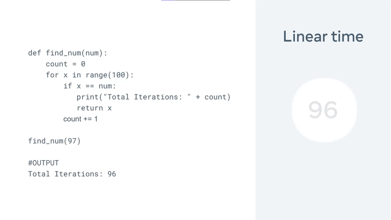
Linear time algorithm
This will grow depending on the size of the input.
For example, if I have an array of numbers with a range of 100, it will run very fast. But if it’s increased to a million, it will take a lot longer to complete. The size in this case, affects the running time of the code.
Logarithmic time algorithm
A logarithmic time algorithm refers to the running time of the inputs against the number of operations.
I can take a linear approach to try to find a number out of 100. Let’s say the number is 97. In a linear equation, it will take 96 iterations before it’s found. This is because it must iterate through each item one by one until it finds the target value.
Using a binary search, I can drastically cut down the iterations and find it on the seven iterations. This is measured by logarithmic time.
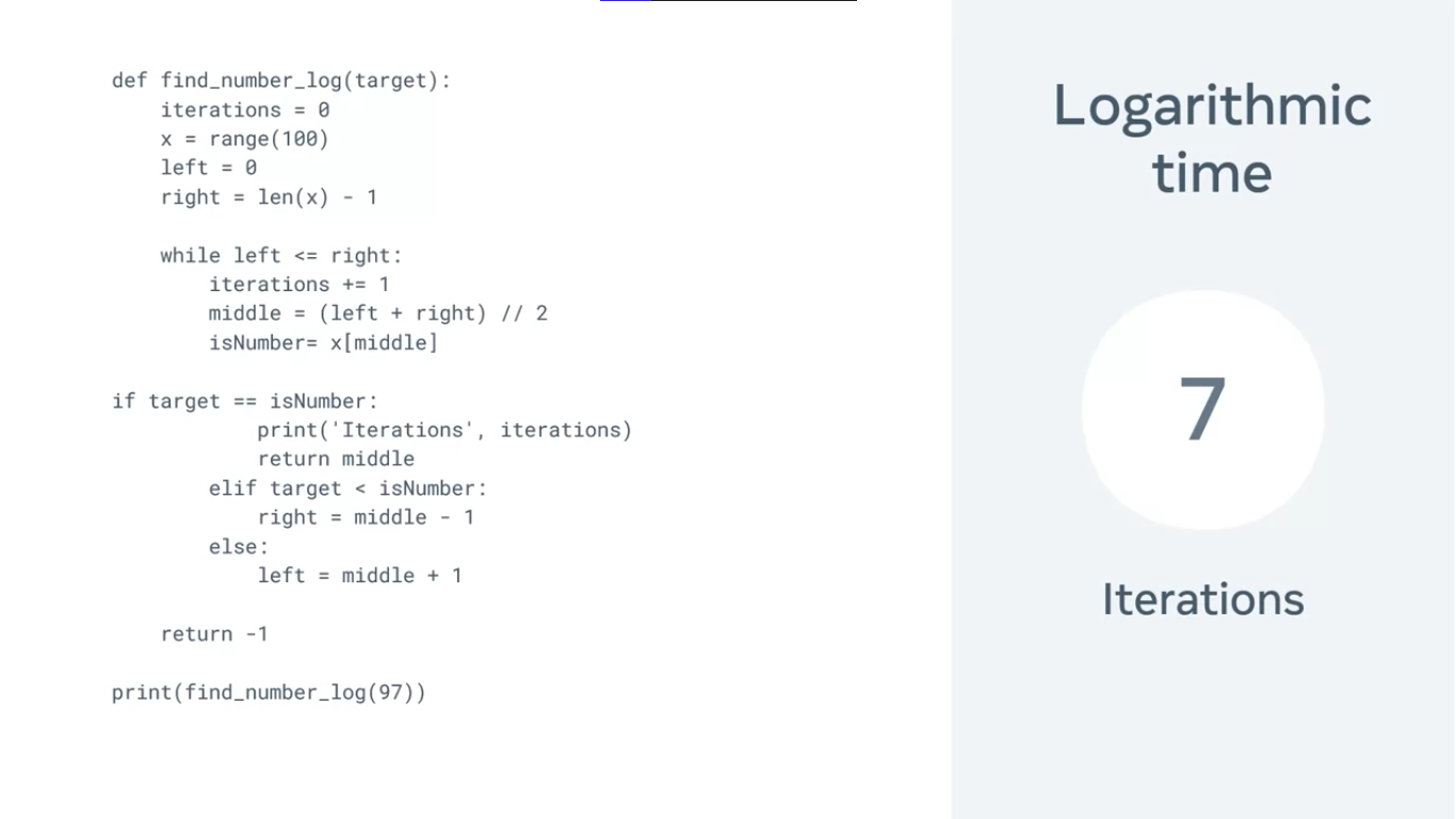
The binary search works by splitting the list into two parts each time to check if a target is less than or greater than one.
Quadratic time
Quadratic time refers to a linear operation of each value of the input data squared. This is often a nested list.
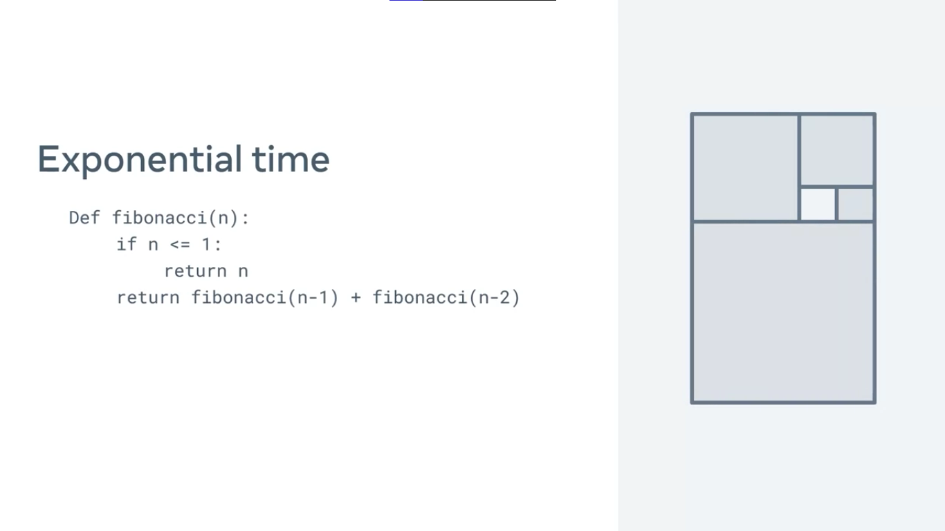
Exponential time
which is an algorithm that doubles with each iteration.
The Fibonacci sequence is a prime example of this.
Intro to Big-O notation
Big-O
Big O notation is a fundamental concept in computer science and programming that helps you analyze and describe the efficiency of algorithms. It provides a standardized way of expressing how the runtime or resource usage of an algorithm grows as the size of the input data increases. This guide will explain Big O notation in simple terms with easy-to-understand Python examples.
What is Big O Notation?
Imagine you are cooking pasta, and you want to determine how long it will take to boil a pot of water. You might consider factors like the size of the pot, the power of your stove, and the amount of water you need to heat. Similarly, in computer science, algorithms are analyzed based on their efficiency when dealing with different sizes of input data.
Big O notation is a mathematical notation that describes the upper bound or worst-case scenario for the time complexity of an algorithm. It helps us answer questions like:
- How does the runtime of an algorithm change as the input data gets larger?
- How does an algorithm scale with increased input size?
Big O notation is written as “O(f(n)),” where “f(n)” is a function that represents the relationship between the input size (usually denoted as “n”) and the algorithm’s runtime or resource usage.
Common Examples of Big O Notation
Let’s explore some common examples of Big O notation using Python code:
O(1) - Constant Time
In algorithms with constant time complexity, the runtime does not depend on the size of the input data. It remains constant, making it the most efficient scenario.
Example: Accessing an element in an array by its index.

No matter how large the array is, accessing an element by its index takes the same amount of time. The runtime is constant, and we denote it as O(1).
O(n) - Linear Time
Algorithms with linear time complexity have a runtime that grows linearly with the size of the input data. This means that if the input data doubles in size, the runtime also doubles.
Example: Searching for a specific value in an unsorted list.
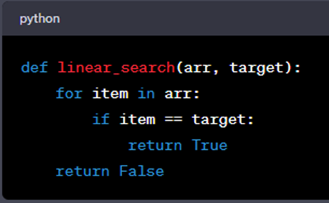
As the size of the list (arr) increases, the number of iterations the loop performs also increases linearly. Therefore, this algorithm has a time complexity of O(n).
O(n^2) - Quadratic Time
Algorithms with quadratic time complexity have runtimes that grow with the square of the input size. As the input data size increases, the runtime increases quadratically.
Example: Bubble Sort, a simple sorting algorithm.
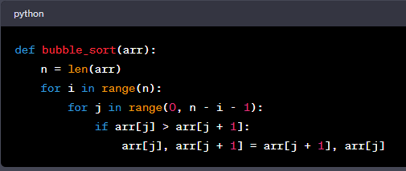
Bubble sort has a time complexity of O(n^2). As the size of the input list (arr) increases, the number of comparisons and swaps grows quadratically.
O(log n) - Logarithmic Time
Algorithms with logarithmic time complexity have runtimes that grow logarithmically with the size of the input data. Logarithmic time complexity is considered very efficient.
Example: Binary search in a sorted list.
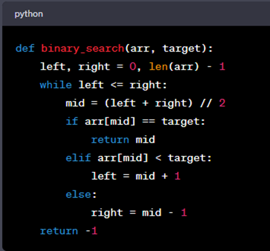
Binary search drastically reduces the search time as the size of the sorted list (arr) grows. It has a time complexity of O(log n).
A Quick Breakdown
-
Fastest:
- O(1) - Constant Time: Lightning-fast! The algorithm’s speed doesn’t depend on how much data you have. It’s like finding your favorite book on a perfectly organized bookshelf – it takes the same amount of time, whether you have 10 books or 1,000 books.
-
Pretty Fast:
- O(log n) - Logarithmic Time: Still quite speedy! It grows slowly as you add more data. Think of it as finding a name in a phone book by repeatedly splitting it in half – it gets faster even if the phone book gets bigger.
-
Moderate:
- O(n) - Linear Time: Respectable speed! If you have twice as much data, it takes about twice as long. It’s like looking through a list of names one by one to find a match.
-
Slower:
- O(n log n) - Linearithmic Time: It’s faster than quadratic but slower than linear. Comparable to sorting a deck of cards quickly using smart techniques.
-
Slower Still:
- O(n^2) - Quadratic Time: Getting slower as you add data. Like checking every combination of items on a list against each other – not great for large lists.
-
Quite Slow:
- O(2^n) - Exponential Time: Now we’re talking about slow! It grows rapidly as you add data. Imagine a puzzle where you have to try every possible combination – it’s really slow even for small puzzles.
-
Incredibly Slow:
- O(n!) - Factorial Time: The slowest of all! It’s like solving a complex puzzle where the number of possible arrangements explodes as you add more pieces. Practically unusable for large problems.
Why Big O Notation Matters
Big O notation is crucial for several reasons:
- Algorithm Comparison: It allows us to objectively compare different algorithms and choose the most efficient one for a specific task.
- Performance Optimization: Understanding Big O helps identify bottlenecks in code and optimize algorithms for better performance.
- Scalability: Efficient algorithms are vital as applications and data sizes grow.
- Resource Management: In resource-constrained environments, like embedded systems, choosing efficient algorithms is essential.
- Coding Interviews: Big O notation is often tested in technical interviews and coding challenges, demonstrating your ability to analyze and optimize algorithms.
Analyzing Code with Big O Notation
To analyze code using Big O notation, follow these steps:
- Identify the Input Size: Determine what “n” represents in your code, often related to the size of the input data.
- Identify Loops and Iterations: Look for loops in your code, as they often determine the primary factors affecting time complexity.
- Count Operations Inside Loops: Count the number of operations inside each loop that depend on the input size “n.”
- Combine Complexity: If you have nested loops, multiply their complexities to determine the overall time complexity.
- Choose the Dominant Term: In cases of combined complexity, focus on the term with the highest growth rate, as it will dominate the overall time complexity.
- Simplify: Simplify the expression as much as possible by removing constant factors.
By following these steps, you can determine the time complexity of an algorithm and understand how it will perform as the input size increases.
In summary, Big O notation is a fundamental concept in computer science that helps us analyze and compare algorithms’ efficiency. By understanding its basics and applying it to code, you can make informed decisions about algorithm selection and optimization, ensuring your programs run efficiently, even as data sizes grow.
Additional resources
The following resources will be helpful as additional references in dealing with different concepts related to the topics you have covered in this module.
- Programming styles in Python
- Different types of algorithms used in Python
- Introduction to Big-O notation
PythonAlgorithmProceduralBig-OParadigm
Previous one → 4.Errors, Exceptions and File handling | Next one → 6.Functional programming